Thursday, October 6, 2011
Wednesday, September 28, 2011
Wednesday, August 24, 2011
Sunday, August 21, 2011

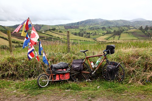
"Using transport bicycles such as this 1950 Schwinn cruiser instead of a car saved me enough money in nine years to pay for three years of overseas travel by bike, boat, and plane. It carries a comfortable payload of 80 lbs in lockable, waterproof panniers." from http://oasisdesign.net/design/principles.htm
Thursday, August 18, 2011
Sunday, August 14, 2011
Thursday, July 14, 2011
For those learning the Soil and Water Assessment Tool (SWAT)...
I suggest checking out this site.
http://www.smm.org/scwrs/tapwaters
http://www.smm.org/scwrs/tapwaters
Wednesday, June 29, 2011
Using r.buffer for watershed analysis
A problem that I ran into when using r.watershed with a masked basin was that the streams were being cut off, and the resulting basin was incorrect.
 |
| Close up of the HUC 10 watershed boundary in black and the streams derived from r.watershed in blue and pink |
 |
| basin resulting from original mask |
To solve this I created a buffer raster of the original raster being used as a mask.
r.buffer input=rioGrandeHUC10mask output=rioGrandeBuffer distances=100
Then, following the grass book
r.watershed -f elev_cm_rioGrande2 thresh=10000 accum=accum_10K drain=draindir_10K basin=basin_10K stream=rivers_10K --o
r.mapcalc "streams_der_30m=if(abs(accum_10K)>100,1,null())"
r.thin streams_der_30m out=streams_der_30m_tmp
r.to.vect -s streams_der_30m_tmp out=streams_der_30m
r.to.vect -s basin_10K out=basin_10K feature=area
Here is the resulting stream
 |
| Streams in green after using a buffer with 100m distance |
r.water.outlet drainage=draindir_10K basin=outlet_O8 easting=170670 northing=270651 --o
r.mapcalc 'outlet_O8=if(outlet_O8==1,1,null())'
 |
| Resulting basin with buffered mask |
Tuesday, June 28, 2011
Wednesday, June 22, 2011
More NHDPlus with GRASS GIS
Here is the flow accumulation grid from the NHDPlus dataset
Here, I take the log of the accumulation again:
r.mapcalc 'log_fac=log(abs(fac)+1)
Extract the streams and convert them to vector:
r.mapcalc 'inf_rivers=if(log_fac>6)'
r.thin input=inf_rivers out=thin_rivers
r.to.vect -s thin_rivers out=inf_rivers
Watershed Analysis using GRASS GIS
After following an exercise provided at <http://www.ing.unitn.it/~grass/docs/tutorial_64_en/htdocs/esercitazione/dtm/dtm4.html>, I have been playing around with different thresholds and flow routing algorithms in GRASS GIS to try to reproduce the National Hydrography Dataset Plus provided by <http://www.horizon-systems.com/nhdplus/>. Below is the NHDPlus elevation, flowlines, and waterbodies data for Puerto Rico. I also added the HUC10 boundary for the Rio Grande de Arecibo basin.
One thing I've been concerned with is representing the waterbodies accurately. From the GRASS GIS book, "The r.watershed module does not require filling of depressions (pits, sinks) in DEM prior to its application because it uses the least-cost algorithm to traverse the elevation surface to the outlet." So, I wanted to test some things.
Firstly, I ran r.watershed using SFD and MFD without filling in the depressions.
Using r.watershed with threshold of 10000 and single flow direction from the command line...
And, the results...
Here is a close up of the southwest corner of the watershed
Taking the log of the accumulation map
Here is the close up from using the MFD method
And taking the log again
Here are the two lakes from the middle of the watershed
Next, I tried r.watershed after filling in the depressions.
The accumulation map after running r.watershed with the depressions filled seems like it would represent the streams better.
However, the resulting streams are not as expected. I tried using each level of filled depressions, and different ways to extract the streams from the accumulation map, but none gave good results.
Here is a map with the streams derived from using r.watershed with SFD on top of the NHDPlus flowlines.
Here is SFD, MFD, and the NHDPlus all in one.
The MFD method using
r.mapcalc 'inf_rivers=if(log_accumulation>6)'
to extract the streams seems to match the NHDPlus flowlines the best.
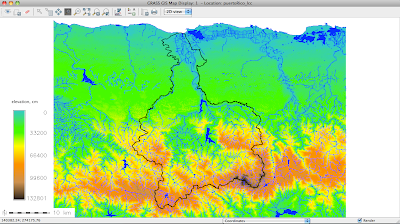 |
| Rio Grande de Arecibo basin in Puerto Rico with flowlines and waterbodies from NHDPlus |
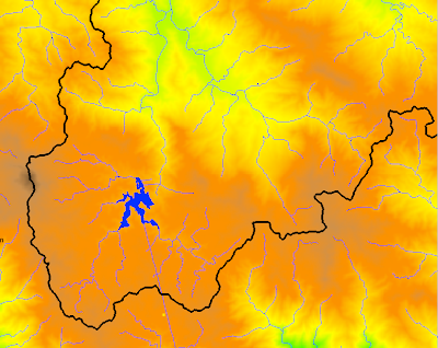 |
| Close up of the southwest corner of the watershed where Lago Garza is located |
 |
| Two lakes in the eastern-central part of the watershed |
Firstly, I ran r.watershed using SFD and MFD without filling in the depressions.
Using r.watershed with threshold of 10000 and single flow direction from the command line...
r.watershed elevation=elev_cm accumulation=rwater_accum10Ksfd drainage=rwater_draindir10Ksfd basin=rwater_basin10Ksfd stream=rwater_streams10Ksfd threshold=10000
And, the results...
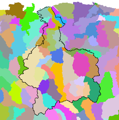 |
| Basin map from using threshold of 10000 and single flow direction |
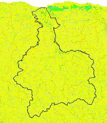 | ||||
| Accumulation map with threshold of 10000 and single flow direction |
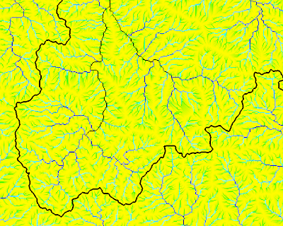 |
| Close up of southwest corner accumulation map for the watershed |
Taking the log of the accumulation map
r.mapcalc 'log_rwater_accum10Ksfd=log(abs(rwater_accum10Ksfd)+1)'
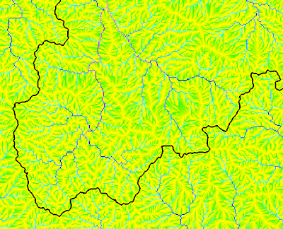 |
| log accumulation |
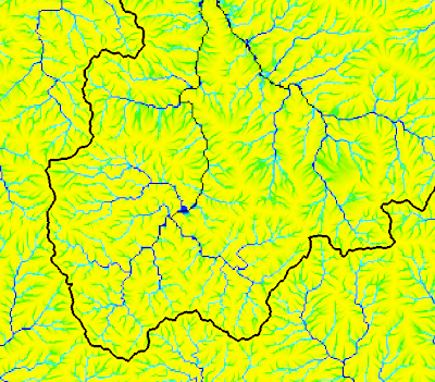 |
| Accumulation map using MFD method |
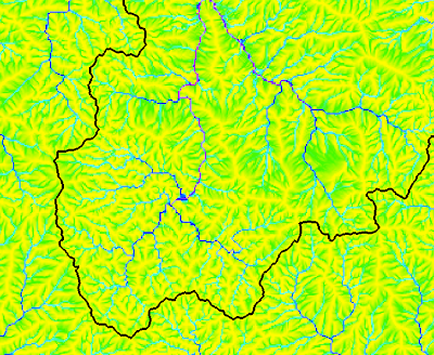 |
| Log accumulation map using MFD method |
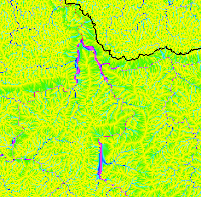 |
| Log accumulation map of the two lakes in the middle of the watershed using MFD method |
Next, I tried r.watershed after filling in the depressions.
r.fill.dir elev_cm el=elev_fill1 dir=dir1 areas=unres1
r.fill.dir elev_fill1 el=elev_fill2 dir=dir2 areas=unres2
r.fill.dir elev_fill2 el=elev_fill3 dir=dir3 areas=unres3
r.mapcalc 'depr_bin=if((elev_cm - elev_fill3)<0., 1, null())'
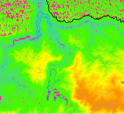 |
| NHD Plus waterbodies outlined in blue and the depression filled raster map shown in fuschia |
The accumulation map after running r.watershed with the depressions filled seems like it would represent the streams better.
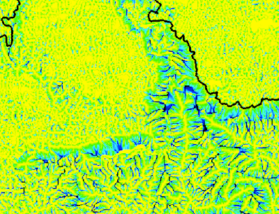 |
| Accumulation map when using depression map and MFD method |
However, the resulting streams are not as expected. I tried using each level of filled depressions, and different ways to extract the streams from the accumulation map, but none gave good results.
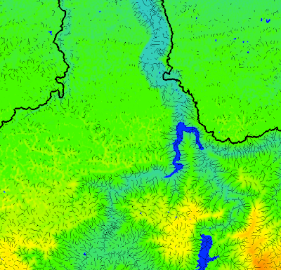 |
| Streams resulting from using a depression filled map |
Here is a map with the streams derived from using r.watershed with SFD on top of the NHDPlus flowlines.
 |
| Streams derived from r.watershed using SFD in fuschia and the NHDPlus flowlines in blue |
Here is SFD, MFD, and the NHDPlus all in one.
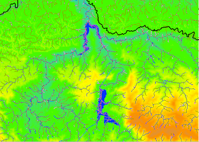 |
| NHDPlus(blue), SFD(magenta), and MFD(light brown) |
The MFD method using
r.mapcalc 'inf_rivers=if(log_accumulation>6)'
to extract the streams seems to match the NHDPlus flowlines the best.
Subscribe to:
Comments (Atom)
